At last! I finally managed to carve out the time to get this out – Water simulations in nuke!

The tool treats the image as a 2D height field, with each pixel as a column of water and a given terrain. The water flows into adjacent pixels based on the height difference and a given user controlled slider. Due to the nature of this method, water can’t travel faster than a pixel per frame, so for large scale images re-timing will be necessary for faster effects.

Flow – Water Simulation in Nuke from Matthew “Rick” Shaw on Vimeo.

Installing

Download from nukepedia.

Simply place the folder in your plugins directory and include the folder in the init.py using nuke.addPluginPath().

Code Breakdown

 

Firstly, let me preface this with a link to the paper that explains the method. It can be hard to dredge through the analysis and formula in these, so I’ll do my best to explain it a bit friendlier here.

Strangely, this requires no blink! So how does it work?

Due to the nature of the method used, we only need to read and write data from adjacent pixels, meaning it can all be achieved with (relatively) simple expressions. We also need to read and write the data at several stages throughout the process, which is a limitation of blink script currently as it only allows one output image. Rather than push and pull to the GPU, we’ll do it all with nuke nodes!

 

The Quick Version

Each pixel is treated as a column of water with a height defined by it’s alpha channel. We imagine each column is connected to it’s eight neighbours by a pipe. We can control the rate of flow by adjusting the size of this imaginary pipe – bigger pipe means more water can flow! There is a formula for calculating the rate of flow through a pipe, and it’s very simple. However, there are a few other factors to consider –  gravity, density and the height difference between the two columns. Altogether, this is still a very easy formula:

 

Additional factors such as atmospheric pressure and external forces can be simulated easily too, by simply adding them to the top line before the division.

However, for our purposes we aren’t going to apply these external forces (at least, not in this version of the tool), which means we can heavily simplify the formula. The height difference will be unique for each column comparison, but everything else is just a multiplier (divisions are just another form of multiplication, 5 / 10 is the same as 5 * 0.1). We can replace them with one single multiplier – Flow Rate.

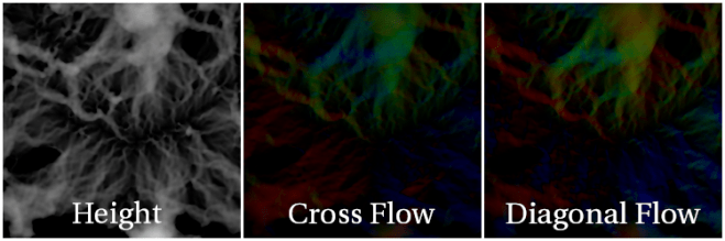
But how to implement this? There are 8 neighbours per pixel (barring edge pixels) and we have four channels for each (rgba), so we’ll use two layers – one for the vertical / horizontal (which I’ll be calling “cross” direction from here on) and one for the diagonals. We’ll store them as follows:

Cross:
-Red:   Flow to the left
-Green: Flow to the top
-Blue:  Flow to the right
-Alpha: Flow to the bottom

Diagonal:
-Red:   Flow to the top-left
-Green: Flow to the top-right
-Blue:  Flow to the bottom-right
-Alpha: Flow to the bottom-left

Now, we can’t just calculate the current flow, simulations require information about the previous frame to accurately simulate the current frame. In our case, each “pipe” has a flow of water going through it, and we need to know whether to accelerate / decelerate it. To do this, we’ll save out the flow from the previous frame, and add it on to our current calculations.

An important thing to note, I’m using frame as our timestep, because that is how it’ll occur in nuke. However, the time period between each calculation could be of any length, often referred to as delta(Δ), so the current update can be written as time(t) + delta time (Δt). In this case, we’d need to multiply by the timestep to keep a consistent rate of flow.

 

Now, each pixel knows it’s outward flow in each direction, but that means it’s opposing side will have an equal but negative value (ie, if 2 units of water are flowing to the left of pixel(5,5), then the outward flow in pixel(4,5) must be -2). To preserve the volume of water in our system, we’ll clamp the outflow to a minimum of 0. If we sum up all the outflow from each pixel and it’s inflow from all it’s neighbours, we’ll know the change in height.

However, we could still have a negative value if the outflow exceeds the inflow. To counter this, we’ll make sure we can’t pour more water out than is currently in the pixel. If we add up the outflow, and it’s greater than the current height, we scale it back til it’s equal. A simple method of doing this is:

min(1, CurrentHeight / TotalOutflow) * Outflow

This way, if the outflow is lower, we’ll only multiply by 1 and get the same result, but if it’s greater it will be scaled back propotionally. Now we can simply add up the inflow, deduct the outflow and we have the amount of change in each column in this timestep. Add it back onto the water, and we’re done!

To allow for the next frame of calculation though, we’ll embed the cross and diagonal flows in the result and write it out as a multi-layer exr. To get a consistent simulation, we need to take in our starting data for the first frame, and switch to the rendered image after that, easily accomplished with a simple switch. And that’s all there is to it! We also calculate colour, but that’ll have to be another post. There’s a lot of room for customisation and expansion in this setup, so hopefully I’ll be revisiting this soon with some modifications and improvements. Have fun!